Scaling laws of translational static friction
How does the static friction \(F_s\) of a crystalline interface scale with contact size \(N\)?
Physics
Commensurate contact (\(\theta = 0\)): Every particle sits at an equivalent substrate site, so all \(N\) particles contribute the same maximum force when the cluster is pushed by one lattice period. The forces add coherently:
where \(F_{1s}\) is the maximum substrate force on a single particle.
Incommensurate contact (\(\theta \neq 0\), small rotation): Particles sit at different substrate phases. As the cluster slides, these forces partially cancel because they point in different directions. For a large, truly incommensurate contact the cancellation gives:
A \(N^{1/4}\) regime is sometimes observed when the cluster contains only a fraction of one Moiré tile, like in a cicular cluster. The crossover is controlled by the Moiré period: the length scale over which the local commensurability repeats.
Note that the exact depenend on \(N\) is not monotonic but it depends on the fraction of Moiré tiles included in the cluster, hence we expect oscillations.
Method
For each cluster size \(N_l\) (controlling \(N\) via cluster_from_params), we compute the translational energy map \(E(x_\text{cm}, y_\text{cm})\) over one substrate period and extract \(F_s = \max |F_x|\) over the grid. We do this for \(\theta = 0\) (commensurate) and \(\theta = \theta_\text{inc}\) (incommensurate). Both circle and hexagon shapes are tested to verify shape independence.
[1]:
import numpy as np
from numpy import sqrt, pi
import matplotlib.pyplot as plt
from time import time

from flake.substrate import substrate_from_params, get_ks
from flake.cluster   import cluster_from_params, rotate
from flake.maps      import translational_map
System setup
Sinusoidal triangular substrate (\(\epsilon = 1\), lattice spacing \(a = 1\)). The cluster lattice spacing equals the substrate spacing at \(\rho = 1\) (commensurate contact).
[3]:
# Sinusoidal triangular substrate, spacing=1.
ks = get_ks(1, 3, 4./3., 0.)

params = {
    'sub_basis':     [[0, 0]],
    'epsilon':       1.0,
    'well_shape':    'sin',
    'ks':            ks,
    'a1':            np.array([1.0, 0.0]),
    'a2':            np.array([0.5, -sqrt(3.)/2.]),
    'cl_basis':      [[0, 0]],
    'cluster_shape': 'circle',
    'N1': 25, 'N2': 25,   # placeholder, overwritten in loop
}

pen_func, en_func, en_inputs = substrate_from_params(params)

# Sanity check: single-particle energy at origin should be -epsilon.
pos_test = np.zeros((1, 2))
e_test   = pen_func(pos_test, np.zeros(2))[0][0]
print('Single-particle E at origin: %.4g  (expected %.4g)' % (e_test, -params['epsilon']))
assert abs(e_test + params['epsilon']) < 1e-6, \
    'Substrate sanity check failed -- check ks values'
Single-particle E at origin: -1 (expected -1)
Grid for translational map
For the sinusoidal substrate we use a Cartesian grid (no unit cell). One substrate period \(\lambda = 2\pi / |\mathbf{k}|\) is sufficient to locate \(\max |F_x|\).
The incommensurate angle \(\theta_\text{inc} = 1.5°\) is small enough to stay near the commensurate contact but large enough to activate the superlubricity regime clearly at these cluster sizes. A larger angle (e.g. \(30°\) for triangular symmetry) would produce deeper superlubricity but is harder to distinguish from a random phase distribution.
[4]:
# Substrate period along x.
period = 2. * pi / np.linalg.norm(ks[0])
n_grid = 50   # 50x50 is coarse but sufficient to locate max |Fx|

xx = np.linspace(0., period, n_grid)
yy = np.linspace(0., period, n_grid)
pos_cm_grid = np.array([[x, y] for x in xx for y in yy])

# Incommensurate orientation: small rotation breaks commensurability.
# 1.5 deg is small enough to stay near commensurate contact but large
# enough to show the superlubricity regime clearly at these cluster sizes.
theta_inc = 1.5   # degrees
Sweep over cluster sizes: circle and hexagon
For each shape and each size \(N_l\) (half-side of bounding box), compute: - \(F_s^\text{comm}\): \(\max |F_x|\) at \(\theta = 0\) (commensurate) - \(F_s^\text{inc}\): \(\max |F_x|\) at \(\theta = \theta_\text{inc}\) (incommensurate)
[5]:
shapes  = ['circle', 'hexagon']
colors  = {'circle':  ('tab:blue',  'tab:orange'),
           'hexagon': ('tab:cyan',  'tab:red')}
markers = {'circle':  ('o', 's'),
           'hexagon': ('^', 'D')}

# Log-spaced sizes: Nlattice ~ 4 to ~100: Nparticle~10 to ~10 000.
Nls = np.unique(np.round(10**np.linspace(0.6, 2, 100)).astype(int))
print('Nl range: %i to %i  (%i sizes)' % (Nls[0], Nls[-1], len(Nls)))

results = {}   # results[shape] = {'Ns_comm', 'Fs_comm', 'Ns_inc', 'Fs_inc'}

for shape in shapes:
    params['cluster_shape'] = shape
    Ns_comm = np.zeros(len(Nls), dtype=int)
    Fs_comm = np.zeros(len(Nls))
    Ns_inc  = np.zeros(len(Nls), dtype=int)
    Fs_inc  = np.zeros(len(Nls))

    t0 = time()
    for i, Nl in enumerate(Nls):
        params['N1'] = params['N2'] = int(Nl)
        pos = cluster_from_params(params)
        N   = pos.shape[0]

        # Commensurate: no rotation, direct reference-frame positions.
        r = translational_map(pos, en_func, en_inputs, None,
                              n_grid, n_grid,
                              pos_cm_grid=pos_cm_grid, n_jobs=1)
        Fs_comm[i] = r['force'][:, 0].max()
        Ns_comm[i] = N

        # Incommensurate: pre-rotate pos before calling translational_map.
        pos_rot = rotate(pos, theta_inc)
        r = translational_map(pos_rot, en_func, en_inputs, None,
                              n_grid, n_grid,
                              pos_cm_grid=pos_cm_grid, n_jobs=1)
        Fs_inc[i] = r['force'][:, 0].max()
        Ns_inc[i] = N

        if i % 10 == 0:
            print('%s  Nl=%3i  N=%5i  Fs_comm=%.4g  Fs_inc=%.4g'
                  % (shape, Nl, N, Fs_comm[i], Fs_inc[i]))

    results[shape] = {'Ns_comm': Ns_comm, 'Fs_comm': Fs_comm,
                      'Ns_inc':  Ns_inc,  'Fs_inc':  Fs_inc}
    print('%s done: %is' % (shape, int(time() - t0)))
Nl range: 4 to 100  (64 sizes)
circle  Nl=  4  N=   19  Fs_comm=53  Fs_inc=51.8
circle  Nl= 14  N=  199  Fs_comm=555.1  Fs_inc=428.9
circle  Nl= 24  N=  583  Fs_comm=1626  Fs_inc=700.6
circle  Nl= 34  N= 1159  Fs_comm=3233  Fs_inc=345.6
circle  Nl= 47  N= 2221  Fs_comm=6196  Fs_inc=737.5
circle  Nl= 65  N= 4243  Fs_comm=1.184e+04  Fs_inc=556.5
circle  Nl= 91  N= 8281  Fs_comm=2.31e+04  Fs_inc=1216
circle done: 95s
hexagon  Nl=  4  N=   37  Fs_comm=103.2  Fs_inc=97.24
hexagon  Nl= 14  N=  547  Fs_comm=1526  Fs_inc=652.9
hexagon  Nl= 24  N= 1657  Fs_comm=4622  Fs_inc=1249
hexagon  Nl= 34  N= 3367  Fs_comm=9393  Fs_inc=789
hexagon  Nl= 47  N= 6487  Fs_comm=1.81e+04  Fs_inc=1154
hexagon  Nl= 65  N=12481  Fs_comm=3.482e+04  Fs_inc=324.7
hexagon  Nl= 91  N=24571  Fs_comm=6.854e+04  Fs_inc=2626
hexagon done: 207s
Single-particle reference
\(F_{1s}\) is the maximum \(F_x\) on a single particle: the atomic-scale friction unit. For a commensurate cluster, \(F_s = N \cdot F_{1s}\) should hold exactly.
[6]:
pos_single = np.zeros((1, 2))
r_single   = translational_map(pos_single, en_func, en_inputs, None,
                                n_grid, n_grid,
                                pos_cm_grid=pos_cm_grid, n_jobs=1)
F1s = r_single['force'][:, 0].max()
print('F1s (single particle) = %.4g' % F1s)
F1s (single particle) = 2.79
Scaling plot: all shapes together
[7]:
fig, ax = plt.subplots(dpi=150, figsize=(6, 4))

for shape in shapes:
    c_comm, c_inc = colors[shape]
    m_comm, m_inc = markers[shape]
    d = results[shape]
    ax.plot(d['Ns_comm'], d['Fs_comm'],
            marker=m_comm, ms=3, ls='none', color=c_comm,
            label=r'%s comm. ($\theta=0$)' % shape)
    ax.plot(d['Ns_inc'], d['Fs_inc'],
            marker=m_inc, ms=3, ls='none', color=c_inc,
            label=r'%s incomm. ($\theta=%.1f°$)' % (shape, theta_inc))

# Reference lines anchored to the data (not to F1s for the sqrt line,
# to allow for the finite-size offset at small N).
Nc = results['circle']['Ns_comm']
ax.plot(Nc, F1s * Nc,
        '--k', lw=0.8, label=r'$F_s \propto N$ (exact for comm.)')
ax.plot(Nc, 2. * (results['circle']['Fs_inc'][0] / Nc[0]**0.5) * Nc**0.5,
        ':k', lw=0.8, label=r'$F_s \propto N^{1/2}$')
ax.plot(Nc, 6. * (results['circle']['Fs_inc'][0] / Nc[0]**0.25) * Nc**0.25,
        '-.k', lw=0.8, label=r'$F_s \propto N^{1/4}$')

ax.set_xscale('log')
ax.set_yscale('log')
ax.set_xlabel(r'$N$')
ax.set_ylabel(r'$F_\mathrm{s}$  [$\epsilon/a$]')
ax.legend(fontsize=7, ncol=2)
ax.set_title('Structural superlubricity: scaling laws  (theta_inc=%.1f deg)' % theta_inc)
plt.tight_layout()
plt.show()
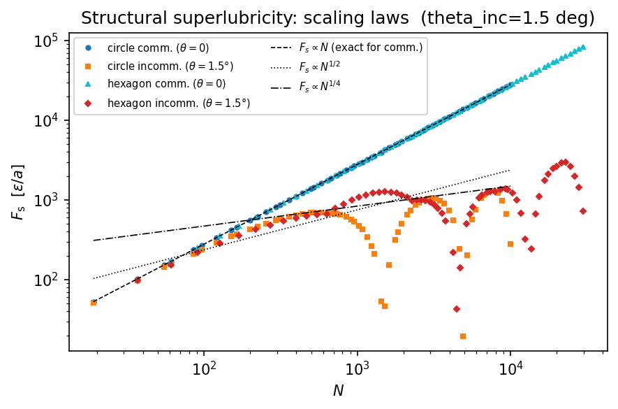
As expected:
Commensurate: \(F_s\) grows linearly with \(N\), matching \(F_s = N \cdot F_{1s}\) exactly.
Incommensurate: \(F_s\) grows sublinearly. At large \(N\) the data approach \(\sqrt{N}\); at small \(N\) (cluster smaller than one Moiré tile) a steeper \(N^{1/4}\) behaviour is sometimes visible. Non-monotonic oscillations at intermediate \(N\) are related to the number of complete Moiré tiles fitting in the cluster — each additional tile contributes a nearly-zero net force increment.
References
[1] Dietzel et al., PRL 111, 235502 (2013) – scaling laws of structural lubricity
[2] Koren & Duerig, PRB 94, 045401 (2016) – moiré scaling in twisted graphene
[3] Panizon, Silva et al., Nanoscale 15, 1299 (2023) – frictionless nanohighways
[4] Dienwiebel et al., PRL 92, 126101 (2004) – superlubricity of graphite
[5] Cihan et al., Nat. Commun. 7, 12055 (2016) – structural lubricity under ambient conditions
[6] Vanossi et al., Nat. Commun. 11, 4657 (2020) – structural lubricity review